Menu
Version 0.0.3
GradieX — Python Library
The gradiex package wraps the float32 engine and adds a matplotlib plotting layer. Training runs entirely in C++: train() hands the whole dataset to core::Network::train and gets a loss history back.
The bindings were rewritten against the float engine and are no longer v0.0.2’s double sources. python/ is now a package: the extension builds as gradiex._core, and gradiex/__init__.py re-exports it alongside seven diagram types. A 4000-epoch XOR run through Python is bit-identical to the same run in pure C++.
Install
From the release directory. A C++20 compiler is required; numpy and matplotlib are pulled in as dependencies.
cd 0.0.3
pip install .
Or build the extension in place, which is what the test scripts and the examples expect:
python3 setup.py build_ext --inplacesetup.py lists core/*.h in depends. Without that, setuptools time-stamps only the .cpp, and editing a header leaves a stale .so in place — the next run silently tests the previous engine, with no error.
Quick Start
Layers are declared, then built. Nothing is allocated until build(), so an invalid architecture raises a Python exception rather than training incorrectly.
import numpy as np
import gradiex

X = np.array([[0., 0.], [0., 1.], [1., 0.], [1., 1.]])
Y = np.array([[0.], [1.], [1.], [0.]])

gradiex.seed(42)                       # reproducible weight initialisation
net = gradiex.Network(learning_rate=0.5, batch_size=4)
net.add_hidden(8, input_size=2, activation="tanh", init="xavier")
net.add_output(1, activation="sigmoid", loss="mse")
net.build()

history = net.train(X, Y, epochs=4000, shuffle=True, seed=42, plot=True)
print(net.predict([0., 1.]))           # -> array([0.984...], dtype=float32)
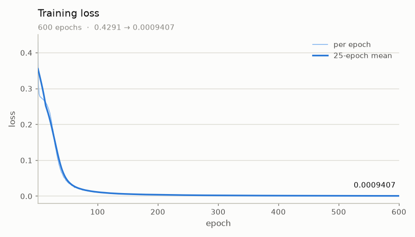
plot=True draws the loss curve when training finishes and leaves the figure on net.last_figure. The history is also kept on net.history, so net.plot_loss() works later with no arguments.
The engine is single-precision end to end. Arrays come back as float32, and float64 input is accepted and cast on the way in. net.learning_rate reads back rounded — setting 0.05 returns 0.05000000074505806.
Plots
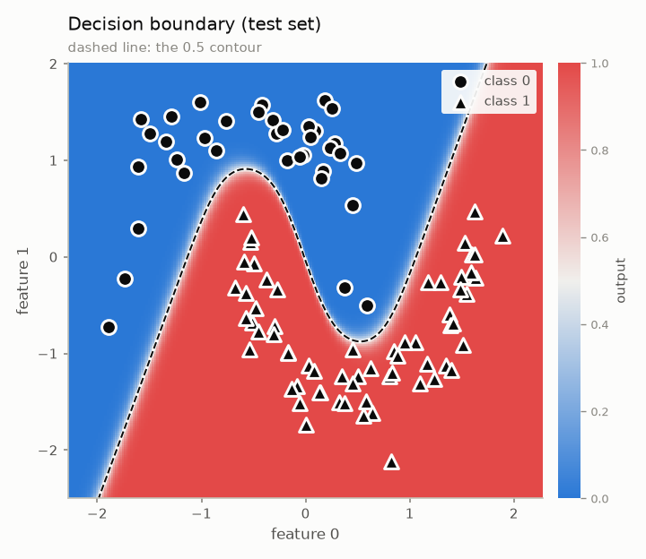
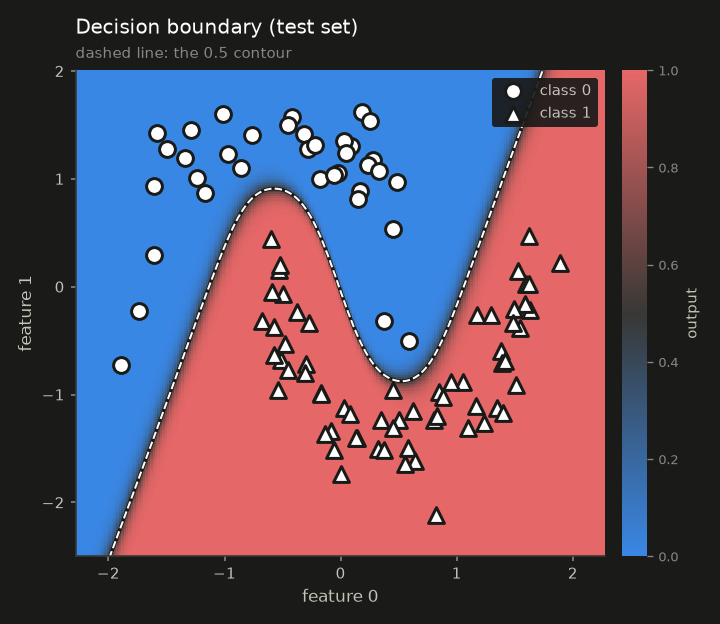
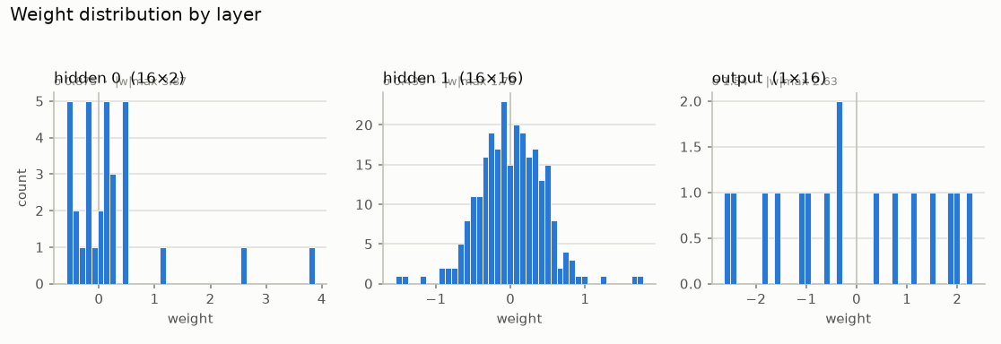
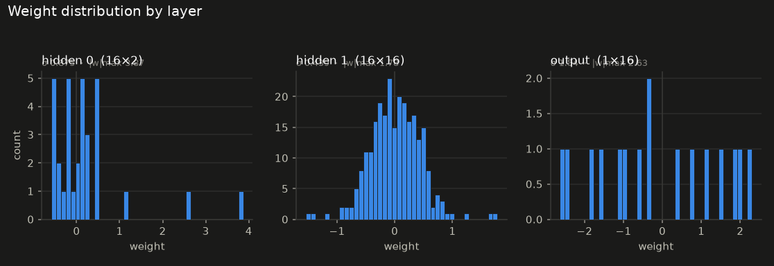
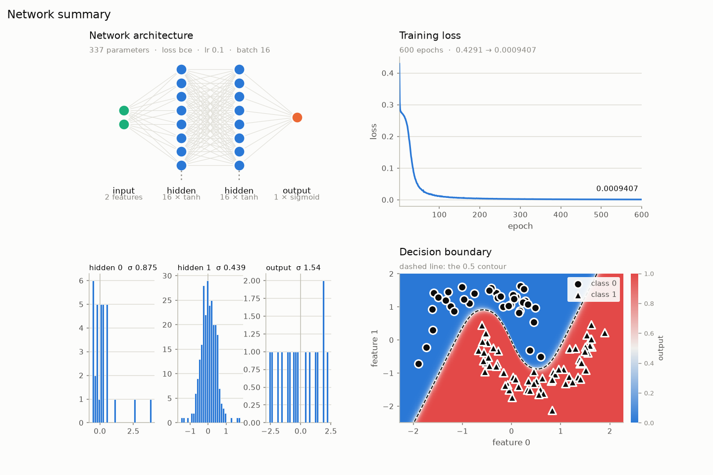
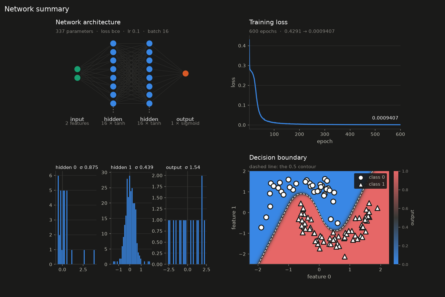
Every figure below was produced by 0.0.3/examples/two_moons.py, which trains a 2 → 16 → 16 → 1 network on two interleaving moons and reaches 100 % train and test accuracy. Each plot takes an optional ax= and returns its figure, so they compose into larger layouts; nothing calls show() unless you pass show=True. Every one accepts theme="light" or theme="dark" — the figures on this page follow the site theme, and each is a genuinely different rendering rather than an inverted image.
Loss curve
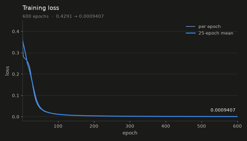
The headline: train(plot=True), or net.plot_loss() at any time afterwards.
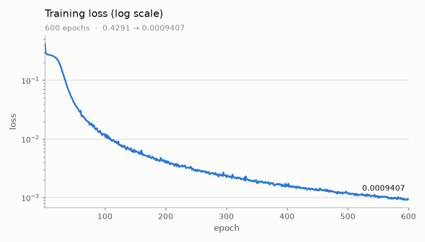
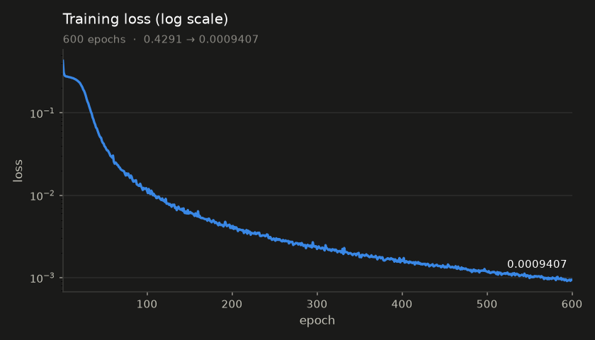
Once a model is fitting well the linear axis flattens out. log=True is usually the more informative view:
Architecture
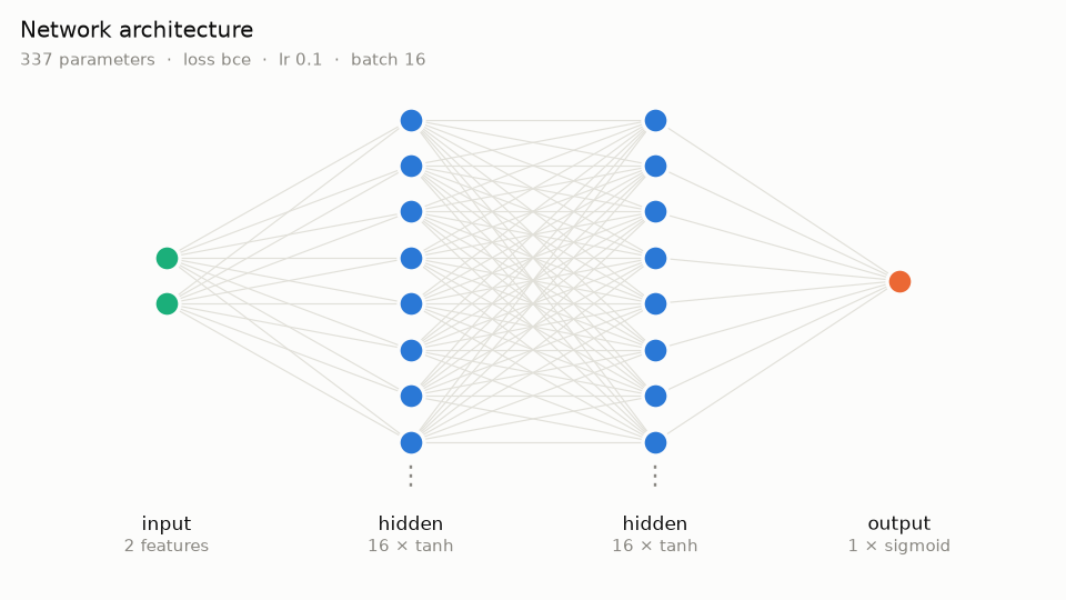
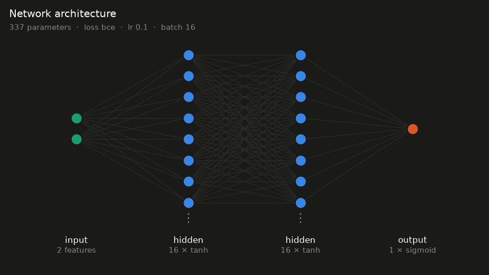
max_nodes are drawn truncated with an ellipsis, and the label always states the true width, so the diagram never misreports the shape it is compressing.Decision boundary
For a network with input_size == 2. A single output is read as a probability and shaded with a diverging ramp about 0.5; several outputs are read as classes by argmax.
Loss landscape
Two random directions are drawn through the trained weights and filter-normalised — each direction row scaled to the norm of the weight row it perturbs — then the loss is measured on a grid of steps along both. The method is from Li et al., Visualizing the Loss Landscape of Neural Nets (2018).
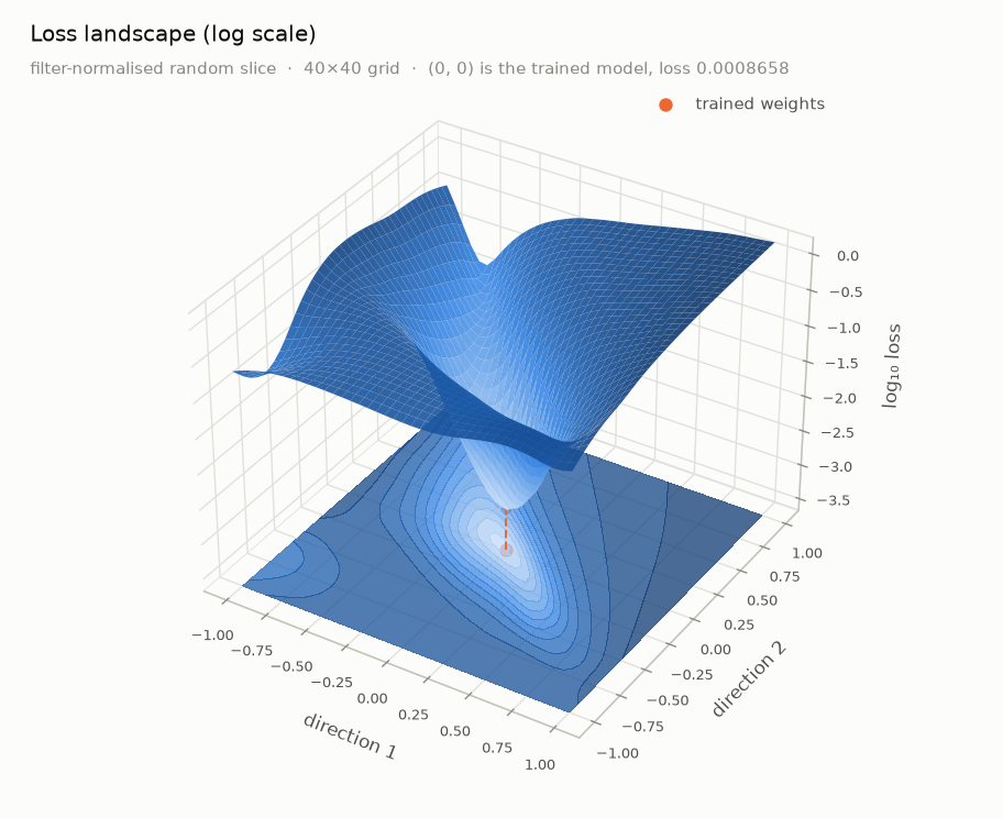
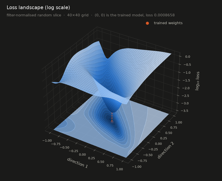
This is a random 2‑D slice of a 337‑dimensional surface. It shows whether the basin is broad and smooth or narrow and ragged; it does not show the path the optimiser took, or where other minima are. A different seed= gives a different slice. The sweep restores the trained weights exactly when it finishes, including if it raises part-way through.
Weights
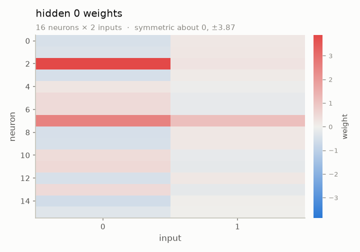
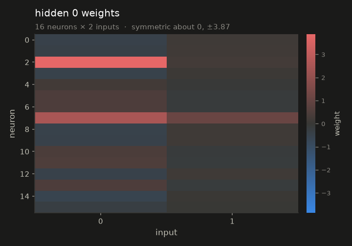
Predictions
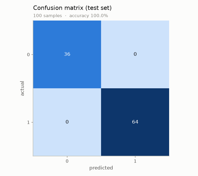
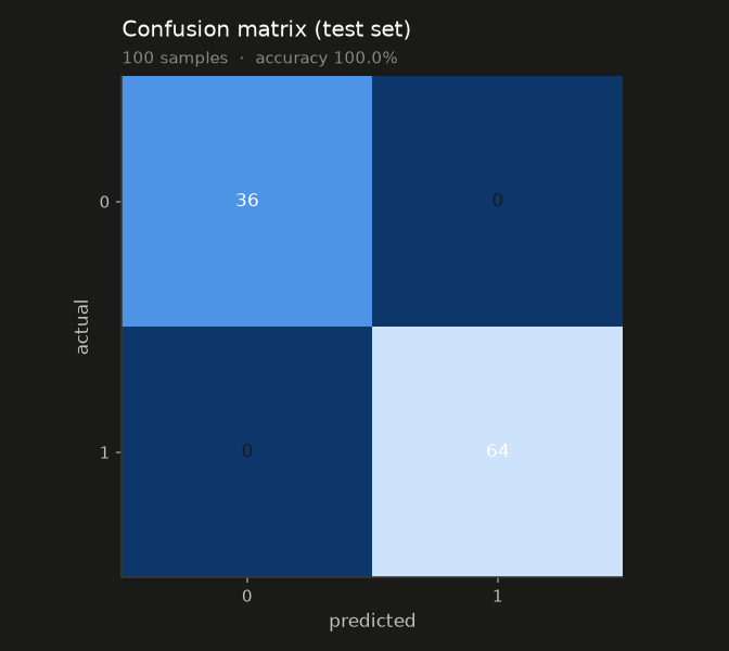
kind="auto" picks between them; pass kind= explicitly to override. Every cell is labelled, so the counts never depend on reading the colour ramp.Summary
Training Runs In The Engine
train() is one call into core::Network::train. There is no per-sample loop in Python, and none in the binding either — the epoch loop, the shuffle, the mini-batching, gradient accumulation and the update rule are all engine code, with the GIL released for the duration.
That is checked rather than asserted. The same 4000-epoch XOR run, same seeds, through both paths:
| Path | First epoch | Last epoch |
|---|---|---|
Pure C++ (core::Network::train) | 0.296616971 | 0.000236376116 |
Python (gradiex.Network.train) | 0.296616971 | 0.000236376116 |
Bit-identical, and the output activations agree to nine significant figures. Two seeds control it: gradiex.seed(n) for weight initialisation, and train(seed=n) for the shuffle.
Watching a validation split means calling train(epochs=1) in a loop, since the engine owns the epoch loop. Each call is still an engine call:
train_curve, held_out = [], []
for epoch in range(600):
    train_curve.append(net.train(X_train, Y_train, epochs=1, shuffle=True, seed=epoch)[0])
    held_out.append(net.evaluate(X_test, Y_test))

gradiex.plot_loss(train_curve, val_history=held_out, labels=("train", "held-out"))API Reference
Construction
| Call | Meaning |
|---|---|
Network(learning_rate=0.01, batch_size=1) | batch_size is how many samples are accumulated before one update: 1 is per-sample SGD, 0 means one batch per epoch. |
add_hidden(width, input_size=None, activation="relu", init="he") | input_size defaults to the previous layer’s width, and is required on the first layer. |
add_output(width, input_size=None, activation="sigmoid", loss="mse", init="he") | Called once, after every hidden layer. |
build() | Constructs the engine and initialises the weights. initialize() is an alias. |
gradiex.seed(n) | Seeds the weight-initialisation RNG. Separate from train(seed=), which seeds only the shuffle. |
Training and evaluation
| Call | Meaning |
|---|---|
train(X, Y, epochs=100, shuffle=False, seed=None, verbose=False, log_every=0, plot=False, **plot_kwargs) | Runs in the engine. Returns the mean loss of each epoch, and stores it on .history. |
train_batch(X, Y) | One engine batch step over these samples. Returns the mean batch loss. |
evaluate(X, Y) | Mean loss over a dataset, engine-side, with no update applied. |
loss(x, y) | Forward one sample, then the configured loss against y. |
forward(x) / predict(x) | One forward pass; returns the output activations. |
Gradient primitives
One method per engine call, for a hand-rolled loop. backward(y) is the convenience form: zero, accumulate, apply.
| Call | Engine method |
|---|---|
zero_gradients() | Network::zeroAllGradients |
accumulate(y) | Network::accumulateGradients |
scale_gradients(factor) | Network::scaleAllGradients |
apply_gradients() | Network::applyGradients |
backward(y) | zero → accumulate → apply, for the sample just forwarded |
Introspection
| Member | Meaning |
|---|---|
weights(layer) / biases(layer) | float32 arrays; weights come back shaped (width, input_size). Negative indices allowed. |
set_weights(layer, values) / set_biases(layer, values) | Overwrite a layer’s parameters. Weights accept (width, input_size) or flat. |
layers | One dict per layer in forward order: kind, width, input_size, activation, init, and loss on the output layer. |
learning_rate, batch_size | Readable and writable, before or after build(). |
num_hidden, input_size, output_size, built | Read-only. |
history, last_figure | The most recent train() history, and the figure plot=True drew. |
Plotting
Each is both a module function taking a network and a method on it. All accept ax=, theme=, title=, figsize= and show=.
| Function | Notable arguments |
|---|---|
plot_loss(history) | val_history=, labels=, smooth=, log= |
plot_architecture(net) | max_nodes= |
plot_weight_distribution(net) | bins= |
plot_weight_heatmap(net, layer=-1) | — |
plot_decision_boundary(net, X, y=None) | resolution=. Requires input_size == 2. |
plot_predictions(net, X, Y) | kind="auto" | "regression" | "classification" |
plot_loss_landscape(net, X, Y) | span=, resolution=, seed=, log=, contours=, elev=, azim= |
summary(net, history, X, Y) | — |
gradiex.THEMES holds the two palettes. matplotlib is imported lazily, on the first plot, so import gradiex does not pay for it.
Names
| Argument | Accepted |
|---|---|
activation | identity (linear), sigmoid, relu, leaky_relu, tanh, swish, gelu |
loss | mse, mae, huber, binary_cross_entropy (bce), cross_entropy (cce), softmax_cross_entropy |
init | zeros, xavier, he |
gradiex.activations(), gradiex.losses() and gradiex.initializers() return these lists at runtime.
activation="softmax" is rejected: its derivative is a Jacobian and the engine implements only the fused form. Use activation="identity" with loss="softmax_cross_entropy", which computes dL/dz = softmax(z) - y directly. predict() then returns logits rather than probabilities.
What The Python Layer Guarantees
The C++ API can reach states that crash or train silently wrong. The binding collects layer specs first and constructs core::Network only in build(), so none of them are reachable from Python.
| C++ hazard | From Python |
|---|---|
| Out-of-range layer index | Indices are assigned by the binding; never passed in. |
| Unfilled layer slots | The network is sized from the specs actually collected. |
| An activation whose derivative does not resolve | Checked against the engine’s own lookup at add_* time, so the two cannot drift. |
| More than one output layer | Refused — accumulateGradients propagates from outputLayers[0] only, so the other heads would train silently incorrectly. |
| Ragged or mis-shaped rows | Every row is length-checked before the engine indexes it. |
Using a network before build() | RuntimeError. |
Tests
python3 python/test_bindings.py    # engine bindings, guards, C++/Python parity
python3 python/test_plotting.py    # every diagram, headless (Agg)
test_bindings.py covers the engine surface and 23 guard cases — each must raise rather than crash. test_plotting.py asserts that every diagram builds a figure with the axes and artists it claims, that the loss-landscape sweep restores the weights exactly (including after a failure mid-sweep), that the directions really are filter-normalised, and that 15 guards raise. It does not assert on pixels; rendering is checked by eye.
The C++ suite is at tests/ — 91 checks, passing under AddressSanitizer and UBSan.